Lap Polished Flats, Spheres and Prismatic Components – Buyers Guide Chapter 3

In this blog the measurement of optics with a Fizeau interferometer that have been lap polished is discussed.

What interferometer is needed to produce good parts? Each manufacturing process requires a specific measurand, the quantity to be measured, to provide the feedback necessary to control the process and produce good parts. In the following posts several applications will be discussed with optional systems highlighted.

Random, Near of Full Sized Tool Polishing

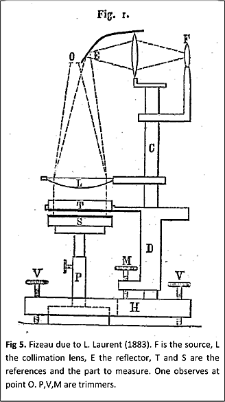
The historic method to manufacture optics has been random polishing on a spindle polisher. The procedure of rough forming the surface

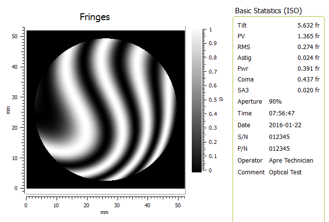
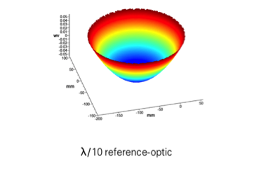
shape, grinding to near polish and then lap polishing has been used for hundred of years. The beauty of lap polishing is the random nature, averaging over large areas of the sphere, which self corrects, and lead to high quality surfaces. Further the mid-spatial frequency ripples, the residual surface features remaining after the removal of 36-Zernike polynomials, tends to be suppressed due to averaging. There are limits and caveats as always, yet in general these are reasonable assumptions. Thus the measurand is simply the shape of the surface as defined by 36 Zernike polynomial coefficients.

The Old Zygo® Mark II Optics Sufficient

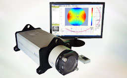
Since the meaurand is simply low spatial frequency shape, in this application, a continuous zoom imaging interferometer, with the inclusion of phase measurement is sufficient. This is why the Mark II architecture as been useful for over 35 years, it was sufficient for nearly all optics produced until this century. The low spatial resolution of the imaging system (no matter the camera resolution), and inherent image distortion of the zoom lens up to ~2%, and slope induced errors have little effect on measurement uncertainty of flats and spheres when measured at a null fringe condition.

Vibration Tolerant Data Acquisition Important

More important than the optical system for this application is the data acquisition and analysis software. This starts with vibration tolerant phase data acquisition as found in modern systems to report phase data without the influence of the production environment vibration. (We plan to discuss the history and development of vibration tolerant PSI in a future blog.) Further the software must be compatible with standard industry standards including ISO and data formats (.dat formats), and be easy to use.

Upgrading an Old Interferometer Is a Good Option

To stay current and meet the the requirements of lap polished optics there are two choices: Buying new or upgrading. The first option is purchasing a newly constructed system with classic optical components that has a new data acquisition system. The second is simply upgrading a classic system to a modern data acquisition system (with vibration tolerant algorithms). The performance of each will be equivalent, with the upgrade being much less expensive.

Summary

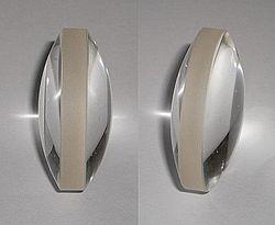
Lap polished Flats, Spheres and Prisms in a normal production environment are sufficiently measured with a continuous zoom system, where the value choice is often a system upgrade.

In the next post we’ll explore what is an appropriate interferometer for transmitted wavefront measurement.

January 22, 2016January 11, 2021

Brief History of the Laser Fizeau Interferometer – Buyers Guide Chapter 2

Click here to read an detailed history

Hippolyte Fizeau, Inventory of the Fizeau Interferometer

In this blog a brief historical outline of the Fizeau interferometer is presented.

Understanding the history of the commercial laser Fizeau interferometer helps to understand the choices available in today’s market. Some systems available today are remnants of historic designs.

Circa 1850: Fizeau Interferometer Invented

Hippolyte Fizeau invented this interferometer configuration for an 1851 experiment that at the time supported the either-drag theory, later disproven by Michelson, leading the way to Einstein’s theory of relativity

1960’s: Lasers

Laser Invented paving way for the laser Fizeau, an unequal path interferometer

1970’s: The architecture is established

The first commercial laser Fizeau interferometer, named for George Hunter the designer

Zygo® invents basic system architecture with sensor (mainframe) and reference (transmission sphere/flat) – the GH Interferometer in 1974.
Zygo® employs twin-spot alignment, with continuous zoom/rotating ground glass imaging design to accommodate low resolution (Vidicon camera) and off the shelf zoom lens (Mark II, in 1978).
Fringe following data acquisition introduced to replace visual fringe evaluation.
Bell Labs invents phase measuring interferometry on a 32X32 array data acquisition using a Vidicon camera, and PDP 8 rack mounted computer.

1980’s: Data acquisition improvements

Digital detectors (up to 256X256 by the late 1980’s), CCD/CID, and workstation computers introduced.
Carrier fringe and four camera simultaneous phase measurement invented (SPMI) for vibration insensitive data acquisition.

1990’s: Software advances

The First Phase Measuring Interferometer at Bell Labs

Enhanced graphics and additional results with faster processing in lower cost personal computers, primarily driven by Wyko and followed by Zygo®
CCD’s with 512×512 pixels introduced – no changes to the ground glass-continuous zoom historic imaging design

2000’s: Data Acquisition and illumination Improved

4D Technologies and ESDI successfully commercialize SPMI
Asphere interferometer introduced: Stitching (QED), Fizeau Scanning (Zygo®)
1KX1K custom imaging driven by deterministic, computer controlled spot polishing
Push to better imaging systems in custom designs
Lower spatial coherence illumination (ring) introduced to improve measurement accuracy

2010’s: MegaPixels + Low Ray Trace Errors + Improved imaging

First newly designed interferometer optical systems that break the ground glass-continuous zoom historic design for high-resolution, low distortion imaging plus minimized ray-trace errors for improved accuracy with steeply sloped wavefronts from mild asphere optics
Sub-nyquist (ESDI) asphere interferometer introduced

2020 and Beyond: Light Sources and Software

Lasers have dominated since the 1960’, but their limitations are catching up with them. Vertex back reflection fringes limit measurement accuracy, spurious fringe mask mid-spatial frequencies, and lasers are unable to measure domes, plates, prisms due to back surface reflections.

To overcome these limitations low coherent sources have been introduced. Delay line white light sources minimize the back reflections and spurious fringe problem but are nearly impossible to align, like a standard white light source.

ÄPRE’s Spectrally Controlled Interferometry (SCI) retains the ease of use of a laser with a long coherence mode and then switches to short coherence (white light) mode at camera frame rates. SCI can also measure the cavity distance enabling the measurement of radius of curvature, without the external radius rail, at higher accuracy. SCI looks like the source of the future.

Confused fringes with laser source (left), clean fringes with SCI (right)

SCI source Spectrum (left) produces Interference fringes (right)

Software

The control of the entire measurement process will become possible with every interferometer using the same measurement setup via centralized control without variation user to user. Software will guide the user as to whether a part passes or fails, and databases will track parts through manufacture and data will be reported consistently, all enabling better process control and thus improved parts.

Summary

The Fizeau interferometer has a long history and promising future. Contact ÄPRE to discuss your interferometery needs to apply the best source + interferometer to your application.

In the next post we’ll explore what is an appropriate interferometer for lap polished flats, spheres and prismatic components.

January 21, 2016March 13, 2018

Fizeau Interferometer Buyers Guide – Chapter 1

The many laser Fizeau interferometer choices make selection confusing.

You don’t want an laser Fizeau interferometer. You just want optics that meet specification, and your Fizeau interferometer helps you do just that. Yet choosing the right interferometer can be confusing. Just consider the choices:

Data Acquisition

PSI, IPMI, or Carrier Fringe, or wavelength tuning, vibration insensitive, vibration tolerant, multi-surface, scanning Fizeau, stitching…

Illumination

high-coherence, low-coherence or partial coherence (ring)

Wavelength

633nm, 1.06um, 3.39um, 1550nm, 10.6um, 650nm, and many others.

Imaging

zoom, discrete, and fixed magnification, plus ground glass or coherent

Detectors

256K, Mega or multi-mega pixel detectors, and then their is CCD or CMOS

System Configurations

Common path, off-axis, high-slope, steep surface, mid-spatial frequencies

Software Analysis

Zernike, slope, ISO, masking, frequency filters, box filters, and a plethora of others

Applications

wavefront, surface, radius of curvature, homogeneity, wedge, corner cubes and …

The combinations are hard to keep track of let alone configure to your specific requirements and budget. So over the next few weeks we will be running a series of blogs to offer some guidance and insight regarding what is important depending on your application.

In the next post we’ll set the stage with a brief history of optical test interferometry.

October 19, 2015January 4, 2018

SPIE: Optifab Rochester NY

It was great making new acquaintances and meeting old friends in Rochester. Optifab continues to be a premier event for optical manufacturers and equipment makers alike. Even the autumn weather did not disappoint.

The REVEAL v1.3 reception was excellent! The new features and capabilities struck a positive cord regarding ease of use and functionality. Especially of interest is REVEAL’s unique reporting function. The ability to create a custom report template for each customer, and not just print out a screen dump, makes shipping documentation easier and meaningful at the same time.

Upgrades to classic interferometers continues to be a hot item. Several times old friends stopped by to say hello, to learn that a useless interferometer they had sitting in a corner could be easily resurrected, with improved performance, and at a low cost.

We can feel the momentum building as REVEAL powers new OEM interferometer applications and the easy upgrade of classic interferometer. Let us know how we can help with your optical test interferometry needs.

February 26, 2015January 4, 2018

Photonics West – REVEAL & 12″ Fizeau

We had an exciting and active Photonics West this year.

Co-exhibiting with Davidson Optronics we demonstrated Davidson’s new 12″ interferometer, designed by Äpre Instruments with Davidson, for Davidson’s manufacture and sales. ÄPRE performed all the sensor’s optical, optical mechanical design, system electronics, firmware and software, which of course runs on REVEAL™. This was an exciting project and a good example of our capabilities. Designed in 13 months, it was a pleasure working with Davidson on this project.

Our OEM REVEAL™ software was a big hit! Both as a basis for interferometer upgrades as well as OEM applications.

We also demonstrated a $44,500 optical profiler running on REVEAL™. It can measure large, >150 mm diameter surfaces, or small optics depending on the configuration.

We look forward to meeting you at our next tradeshow.

September 9, 2014

Measurement Repeatability: How much is enough?

How many times have you looked at an interferometer specification and to see a number under Simple Repeatability like λ/10,000 and wondered, “Who cares?” Add to this the long footnotes that tell you how the number was obtained, usually through significant averaging, idealized short interferometer cavities (think 1 mm) and statistics from around 30 measurements. Then the RMS is reported which further averages the data. When you consider how an interferometer is used, a 1 mm cavity coupled with averaged data seems irrelevant.

The escalation of specifications like Simple Repeatability has occurred for a couple reasons: First, some purchasing departments buy purely on specification, and if one system’s Repeatability is lower than another system’s…guess who wins. And second, there is potentially a bit of pride in saying our numbers are the best. Notice the reason is not to tell the user what is important, or what is “good enough”.

Repeatability considerations:

Repeatability only applies to each particular measurement situation. Environment, part interactions with the interferometer ( for example stray light), and the interferometer data acquisition play a role.
Another variable not seen on specification sheets is REPRODUCIBILITY. It does not appear because it can only be measured for a particular measurement in the use environment. Reproducibility is the variation due to operator to instrument interactions (tilt fringes for example), long term environmental variations, fixturing induced errors and other unforeseen complications.
In many industries a GR&R test is used to quantify and separate the contributions of repeatability and reproducibility. The typical target for a GR&R test is ≤10% (combining both contributions) of the measurement tolerance. For a λ/10 P-V surface that means a λ/100 P-V, or ~λ/500 RMS GR&R. A far cry from λ/10,000 reported.
This does not mean that ~λ/500 RMS GR&R is easy to achieve. When considering real life conditions ~λ/500 RMS GR&R can be very hard to achieve. The important issue is knowing what your GR&R is compared to the desired tolerances to see if the measurement is meaningful.

From a metrology viewpoint repeatability as reported on specification sheets is meaningless. GR&R is the meaningful parameter to use for your measurement set up and tells the true story.

What other specification really matter and why?

Let us know what you would like discussed.

Thank you for reading.

April 22, 2014January 4, 2018

Which Result is “Right”?

What accuracy can be achieved with an Interferometer?

Instrument correlation sets a performance base line for metrology instruments. When parts are manufactured and shipped, correlation between vendor and customer is expected. If metrology systems do not correlate arguments ensue regarding who is right.

Several years ago I received a call from a quality manager. He was unhappy with the results of a correlation study comparing several interferometers in his factory. The test was simple. He manufactured several parts and measured them on the various systems. Each system was stand-alone and had its own set of λ/10 accuracy transmission sphere reference optics. The temperature throughout the factory was held to ± 0.2C and only trained operators were used. Surprising to the QC engineer, the measurements only agreed to λ/5. 2X worse than expected.

Why?

There is a common misunderstanding that since λ/10 reference-optics are accurate to λ/10 that instruments using them will correlate to λ/10. Yes the reference-optics are accurate the λ/10, that is ± λ/10. Therefore when you compare results they can correlate too much better than λ/10 (down to the instrument noise if low pass filtering is applied) or differ by λ/5, just what the quality manager noticed.

How does this affect vendor quality control and customer inspection?

When measuring spherical and flat optics the measurement uncertainty to first order is determined by the reference optics accuracy. For aspherical optics this is not the case, and might be the subject of a future blog. So lets keep it simple and assume spherical and flat optics are being manufactured. In practice the application of error sources is somewhat more complicated for spherical optics, the following argument is true for flat optics and mostly true for spherical optics. For flats the lowest order error is power, for spheres the errors of interest are 3rd order Spherical, Coma and Astigmatism.

The Vendor

The manufactured part has a tolerance; we’ll assume is λ/2 for this example. When the part is measured the result includes the part shape error and the reference optic uncertainty, an unknown but within ± λ/10. Therefore if the measurement is on the high side it can be as poor as + λ/10 worse, and if on the low side – λ/10 worse than measured.

To be assured the part meets specification it must be manufactured to ± λ/10 tighter tolerance, shown in figure 1. Now the manufacturer knows the part is within tolerance, and is certain they are shipping a good part.

The Customer

Upon receiving the part the opposite is true. The customer has no knowledge of the sign of the reference surface optics error. Therefore the parts must be accepted if the measured surface error is within the tolerance PLUS the reference surface uncertainty as shown in figure 2. The customer must be certain they would only reject out-of-specification parts, and this means opening up the tolerance based on the reference surface accuracy.

Design Tolerances Must Consider Metrology To Assure Optical System Performance

The summing of these uncertainties and the epistemological problem drives optical specifications to tighter tolerance. At some point, about 2X the reference surface accuracy, meeting specification becomes expensive due to the tightened tolerance window. At this point improving the reference surface accuracy will open up the manufacturing tolerance window decreasing manufacturing costs. Three methods are available to improve reference surface accuracy:

The easy method costs money, purchase ± λ/20 reference optics – or better. This can be cost prohibitive.
Using a three-flat test or a two-sphere test to achieve “absolute” calibration. This works well in theory. Practically the test must be performed with careful attention to alignments to improve the reference surface.
The most recent test is a calibration ball where averaging is used to calibrate a spherical reference surface and has shown promise in well defined conditions.

Good Metrology Practice

Understanding the role of reference surface accuracy in optical metrology leads to improved tolerancing, establishing appropriate test procedures within manufacturing processes, and an approach to minimize disagreements between vendors and customers.

March 21, 2014January 4, 2018

Nothing lasts forever: Interferometer Upgrades

Summary

The main culprit to interferometer failure is a computer crash due to drive failure. The main cost is often lost production due to down time. Planned upgrades of production systems can save hundreds of thousands of dollars in lost production. After 10 years it is best to plan an upgrade of all systems when production will not be affected.

After 10 years of operation over ~95% of interferometer systems will have failed. In ten years operating systems, electronics, and hardware drivers are incompatible with analysis software developed ten years earlier. These factors signal the need to upgrade.

Old Reliable

After years of reliable service it is easy to assume your interferometer will start tomorrow. Decreases in system performance are hard to detect over a long period. Like an aging car that seems adequate until you drive a new one, then you realize how worn the old car is. So what drives interferometer failure, and what must be considered when you upgrade your system?

The main drivers for having a dead interferometer are laser, moving parts (motors and piezos), electronics (driver boards and camera) and computer. The laser is considered a maintenance component and will not be discussed here.

When motors, piezos, cameras or electronic driver and frame grabber boards fail replacements often do not work with the present operating system or analysis software. If a component can be found, software drivers are usually not available. So in all cases the ability to repair an interferometer depends on the computer and software.

Computer Crashes

The main culprit in computer reliability is the “disk drive”. (Solid State and Hard Disk drives reliability are essentially equal) Computers are reliable for 3 years then start a rapid 12% failure rate. A blog post titled “How long do disk drives last?” by Brian Beach; November 12, 2013 presented the data shown here. Computerized interferometers follow the same failure curve.

If a computer drive crashes in the first few years, cost is driven by the time to purchase a new disk drive, installing it and the reloading the drivers and software to bring the system up. The drive upgrade is simplified with a mirrored drive maintained in stock. This is not true for 10-year-old systems. At some point hardware drivers are no longer available, operating systems do not recognize the analysis software and electronics are incompatible with computer busses and interfaces. This is the time for a system upgrade.

Upgrade Cost

The major cost to an interferometer upgrade can be lost production. At a minimum assume one full week downtime to upgrade a system. Depending on utilization and backup test capacity this one-week could be costly. Shipping just $2MM per year through an interferometer will cost ~$8,000 per day in down time, 3X more than an upgrade costs! Considering downtime here are some rules of thumb regarding when to upgrade.

Rules of Thumb to Minimize Cost

Systems Used on Production Critical Path

< 10 years old, drive failure

Action: Replace drive with a mirrored disk drive that is maintained in stock for easy replacement

Time to revive: 1 day

Cost: ~$8,000 lost production if on critical production path and ~$1,000 if not on critical path

5 to 10 years old, failure other than drive

Action: Upgrade system

Time to revive: 10 days to upgrade + 5 days to identify upgrade company

Cost: Upgrade price ($15,000 to $35,000) + ~$110,000 lost production if on production critical path

5 to 10 years old, planned upgrade

Action: Upgrade during annual maintenance cycle (production shutdown)

Time to revive: 7 working days (purchase decision is done before hand and planned for during shutdown)

Cost: Price of upgrade ($15,000 to $35,000)

All Cases (Critical path and NOT on production critical path)

>10 years old, time to plan an upgrade

Action: Upgrade during annual maintenance cycle (production shutdown)

Time to revive: 7 working days (purchase decision is done before hand and planned to minimize shutdown)

Cost: Upgrade price ($15,000 to $35,000)

Minimal Cost, Minimal Risk Plans Summary

<10 years: If drive fails replace with mirrored drive maintained in stock

>10 years: Upgrade during shutdown or when convenient

Conclusion

An interferometer will not last forever, yet with simple planning cost and risk can be minimized. During the first ten years the primary risk is computer drive failure. After ten years the software and hardware architecture becomes obsolete increasing the difficulty to simply fix a failed component or drive. The major cost risk is failure during production. Therefore maintaining a mirrored drive for each interferometer is the best insurance policy up to ten years. After ten years planned upgrades are much less expensive than lost production.