Optical Surface Radius of Curvature

Optical surface radius is a primary control parameter. It must be measured to confirm the optical element meets specification. Spectrally Controlled Interferometry promises a faster and more accurate method to measure surface radius.

Multiple methods are presently used to measure radius.

  • Test plates: A test plate has a pre-measured radius to which the test surface is compared, the difference is power fringes is reported.
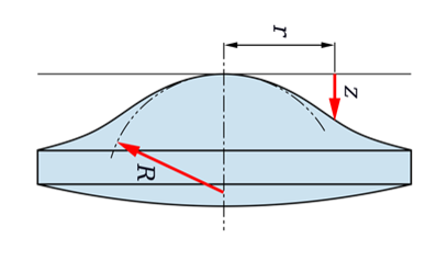
  • Mechanical probe: The sagitta of the lens surface is measured over a fixed diameter, from which radius is calculated. Small changes in sagitta measurement can lead to large errors in reported radii.
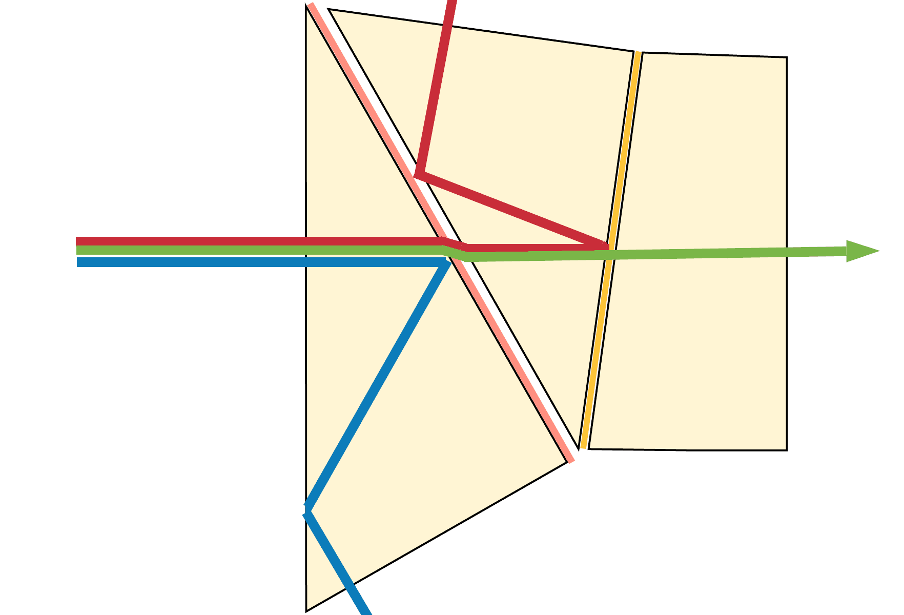
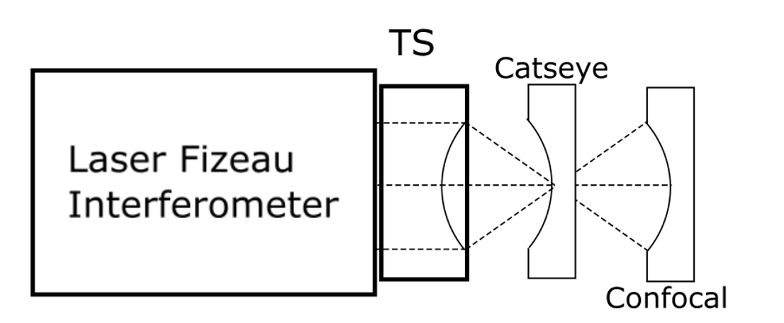
  • Interferometer “Cateye to Confocal”: An interferometer with a transmission sphere (TS) is set up at the catseye position off the surface of interest, and position noted. Then the lens is moved to the confocal position and the position noted. The difference in positions is the radius. PMI interferometers also compensate for any residual power in the measurements due to imperfect positioning. The positions are shown in figure 1.

Interferometer radius measurement is the “gold standard” method today. To achieve this measurement the following additional equipment is needed:

  • Lens mount that allows for free motion along the axis of the lens (Z axis) to micrometer position accuracy
  • Free Z motion over up to a meter, with micro-radian angular alignment to minimize cosine errors.
  • A separate Z position metrology tool. Either a glass scale or a displacement measuring interferometer (DMI) The DMI is the most accurate as it minimizes Abbe offset errors, though it adds environmental uncertainty if not calibrated.
Figure1: The distance between catseye and confocal is the surface radius. Note extra mechanical fixturing and metrology instruments are needed to measure the positions accurately

Spectrally Controlled Interferometry (SCI) Radius Measurement

SCI has a unique combination of four properties:

  • Easy alignment in laser mode
  • Electronically switch to white light mode to isolate fringes to the surface of interest
  • Measures the cavity phase electronically (no mechanical motions)
  • Measures the absolute distance of the measured cavity

SCI Absolute Position Measurement

The SCI source parameters that determine the absolute distance measurement are:

λ0 = The nominal wavelength of the SCI source
Δλ = A tunable source parameter

The absolute distance from the transmission sphere to the optical surface is:

lc = λ20 / 2Δλ   (1)

This combination means SCI can provide all the measurements required for surface radius with neither an additional DMI, nor the precision mechanics to move from Catseye to Confocal position.

SCI Radius Measurement

Since SCI can measure absolute position there is no requirement to measure at two positions. For the first time surface irregularity and radius can be measured at the same time. This also improves measurement accuracy by the elimination of several error sources as discussed below.

SCI Radius is measured by first calibrating the radius of the TS = RoCTS. Then directly measuring the cavity length lc with SCI and calculating the part RoCx from:

RoCx = RoCTS – lc   (2)

Figure 2: Measuring surface radius of SCI requires calibrating the TS radius and then directly measuring the cavity length and calculating the Test Optic radius.

Measurement Accuracy

Repeatability

The foundation of accuracy is repeatability. If a measurement process is repeatable it can then be calibrated to yield accurate results. Repeatability of measurement has been shown to be <0.5 µm for radii in the 20 mm to 175 mm range. This repeatability is better the best measurements with DMI’s.

Accuracy NIST Study

In 2001 NIST ran an experiment to determine the error sources and limits of accuracy for surface radius1. The results of that experiment and error sources are shown in figure 3, along with estimates from Typical DMI and Typical Scale (Glass) radius benches and SCI. 

A key observation is most of the error sources are due to measuring the distance between catseye and confocal. In the NIST study fully 90% of the errors are in this part of the measurement. The same is true for the DMI and Glass Scale. The only difference is the magnitude of the errors that are 16X and nearly 500X greater, respectively, than the NIST study. 

These values are a precaution to users of a DMI or glass scale radius bench to not underestimate the errors in the measurements.

Figure 3: Surface radius error budget for several methods of measurement.

SCI Eliminates the Z Axis Motion Error Sources

No Z motion eliminates the first six error sources (green). Leaving the balance of the error sources that are equal to the Typical DMI set up. SCI can potentially improve the uncertainty to better than the NIST study.

An additional error source is the calibration of the TS radius that also must be added. Since it can be bootstrapp calibrated to the same level a simple doubling of the errors to ~50 nm is expected. 

As of October 2020 SCI can measure surface radius up to 250 nm cavity lengths, and potentially out to 500 mm cavity lengths. 

Summary

SCI promises to replace traditional catseye-confocal lens surface radius measurement by saving time and greatly improving accuracy. It is the go to method for high-performance lens radius metrology.


1 T. Schmitz, A. Davies, C. Evans; Uncertainties in interferometric measurements of radius of curvature, Appeared in Optical Manufacturing and Testing IV, H. Philip Stahl, Editor, Proceedings of SPIE Vol. 4451, 432-447, 2001

Measuring Prisms: Multiple Wavefront Channels In One Setup

Prism Stacks Produce Multiple Wavefronts

Prism stacks are difficult or even impossible to measure with a laser interferometer, yet are easy to measure with Spectrally Controlled Interferometry (SCI). 

Examples of prism stacks for projector imaging systems, displacement measuring, monolithic or assembled component interferometers, and RGB combiners. 

Laser Interferometer Back Reflections

A laser light source interferometers (for example a laser Fizeau) create fringes from every back reflecting surface. In some prism assemblies these are created in multiple channels and are superimposed creating confused interference patterns that are impossible to measurement. 

Spectrally Controlled Interferometry Eliminates Back Reflection 

Spectrally Controlled Interferometry (SCI) can selectively isolate the interference cavity of interest for easy and accurate measurement. And as opposed to white light “delay line” interferometers, SCI is easy to align alignment prior to measurement using its long coherence alignment mode.

Imaging System Prism Stack

In an imaging prism stack the transmitted wavefront passes through several back reflecting surfaces, see figure 1. In this case there are four potential back reflection surfaces. SCI can measure each of these independently if the surface is of interest, or only the transmitted wavefront without corruption. This allows a straight on measurement without tilting or distorting the wavefront.

Figure 1: Schmidt-Pechan Prism. The circled interfaces are areas where back reflections can prevent accurate measurements with a laser interferometer. (ref. https://commons.wikimedia.org/wiki/File:Schmidt-Pechan_prism.svg)

Displacement Measuring Interferometer Components

Interferometers for displacement measurement typically have multiple channels for the test and reference beam path. SCI enables the measurement of each channel independently, without the degrading influence of multiple entry and exit surfaces. To select the measurement channel cavity the polarization is rotated by 90º from one to the other, which is accomplished at the interferometer. [A linear polarized interferometer, where the polarization can be rotated, is used for this application. Contact ÄPRE for more information.]

Figure 2: a-WOW Interferometer for measuring displacement and angle. (ref. Loughridge, Russell & Abramovitch, Daniel. (2013). A tutorial on laser interferometry for precision measurements. Proceedings of the American Control Conference. 3686-3703. 10.1109/ACC.2013.6580402.)

RGB Prism Combiners

RGB (red-green-blue) prism combiners are particularly difficult to measure. The three channels must be separated to measure each path’s transmitted wavefront, yet optically they are co-axial. With a laser interferometer this is impossible, as all the wavefronts overlap, see figure 3. Plus there are multiple back reflecting surfaces that must be eliminated for an accurate measurement. Each channel can be aligned independently in the long coherence align mode. Then selected in the short coherence mode for accurate measurement. 

Figure: 3: Dichroic Prism for RGB selection. The red circle indicate surfaces that reflect back into the interferometer confusing or suppressing the measurement.

Interferometer resolution

Many RGB prism combiners are classed as micro-optics with a less than 6 mm clear aperture. Therefore a standard 4 inch (100 mm), zoomed imaging interferometer with ~400µm image resolution or worse at all zoom magnifications, has insufficient image resolution. A minimum of 60 µm image resolution is required to measure the wavefront of a 6 mm clear aperture prism. 60 µm resolution yields a 100 X 100 image resolution across a 6 mm clear aperture.


Figure4: Image resolution demonstrated for 100 mm aperture interferometer. Airy disk size properly sampled at ≥Nyquist limit is required

NOTE:  This is not 100 X 100 pixels but image resolution. The camera array must be 2X this or a minimum of 200 x 200 pixels AND the imaging optics must produce an airy disk size of 60 µm. At 100 X 100 image resolution 36 Zernike polynomials are accurately calculated. See Figure 4.


Shown in figure 5 is ÄPRE’s S6|HR interferometer with 15 µm image resolution capable of measuring the transmitted wavefront in components to 1.5 mm clear aperture.

Figure 4: ÄPRE S6|HR interferometer with SCI light source for measuring micro-optics including prisms and prism assemblies.

Spectrally Controlled Interferometry Separates the RGB Channels

Again with a laser interferometer the three channels create back reflections simultaneously making the measurement impossible. In the measurement set up (see figure 5) each six prism assembly cavity has three cavity of different optical path lengths. Therefore the distance between the test and reference flat is different for each channel. With SCI each channel is selected one-at-a-time. Typical measurement results with SCI and S6|HR are shown in Figure 6. 

Figure 5: RGB Prism assembly setup with S6|HR Interferometer.
Figure 6″ Typical results measuring an RGB prism assembly with S6|HR and SCI. One setup three results in seconds.


Summary

Prisms assemblies are difficult optical elements to measure. Back reflections from multiple surfaces and multiple channels make laser interferometry incapable of making these measurements. SCI offers an easy to use, accurate method to measure these components for the first time. 

More Applications >

S6|HR Interferometer Specification>

Learn More about SCI>

Applied Optics Paper >

Let’s Talk>

Laser Munich 2017

Jan Posthumas of LaserPeak (on left) and Don Pearson, ÄPRE’s VP Sales (on right)

Don Pearson, our VP Sales and Jan Posthumas, of LaserPeak (ÄPRE Representative) presented ÄPRE’s S100|HR interferometer in Munich this June. Once again we were pleased to meet with, and make new friends while co-exhibiting with the PTB’s HLEM (Hi-Level Experts Meeting) group.

Presented was the S100|HR, part of ÄPRE’s S-Series interferometers with diffraction limited imaging to 50 µm resolution (S50|HR), and all with <0.1% image distortion and <λ/20 retrace errors even at 6.5 fringes/mm.

We were also pleased with the interest in our new SCI based system that electronically remove back reflections from measurements and we look forward to discussing this more in the future.


Photonics West 2017 Introductions

Don Pearson, VP Sales and Takuya Mikami of Okamoto Optics Works discuss ÄPRE’s S100|HR interferometer

It was great to meet many new and old friends in San Francisco at Photonics West. Tradeshows give all of us an opportunity to discuss the challenges and opportunities facing us and discovering how working together we can help each other. Photonics West was no exception.

This year we introduced the latest member of ÄPRE, Don Pearson Vice President Sales. Don comes to ÄPRE with a long history selling and applying interferometers and is known to many in the industry. Previously of Mahr and Trioptics Don is looking forward to meeting you and seeing how we can work together.

We also introduced to Photonics West our S100|HR laser Fizeau interferometer. We are pleased at its reception and how measuring mid-spatial frequencies and form with one instrument is a cost and time savings. Plus accurately measuring 5X more slopes gets the final figuring process started sooner, saving time.

Contact us to discuss how we might work together.

Fizeau Interforometer: To Zoom or Not to Zoom…

In this blog we explore the camera array size required to accurately measure Zernike polynomials in a laser Fizeau interferometer, and thus determine when a zoom system is important. (Hint: Zoom is a historical artifact)

Is a Zoom System Required?

Recently we were asked to provide a system with 4X zoom imaging to accommodate a 25 mm part in a 100 mm system. The thinking being to accurately measure a small part a zoom system is required. It is important to first understand what is the measurand, the quantity measured. In this case the customer wanted to measure and correct alignment errors as indicated by Zernike polynomial terms.

A zoom system adds complexity and cost, plus it can make calibrating the aperture size (pixel size) more complicated. A zoom also matches the image size to the camera, maximizing the pixel count active in a measurement. This raised the question, “How important is pixel count for measuring 36 Zernike terms accurately?” In this case accurate meant up to λ/10 P-V.

Camera Array Size Simulation

Using ÄPRE’s REVEAL software we simulated a measurement by building an artificial surface in the Zernike surface generator. The generator can be set for any pixel array size. Three pixel array sizes were simulated: 512 X 512 (1X zoom), 128 X 128 (4X zoom), and 64 X 64 (8X zoom). See figure 1 for examples of the 64 X 64 and 512 x 512 array data.


figure 1: Simulated data and represented in a 54 x 64 array (left) and 512 x 512 array (right)

The input values of the 36 Zernike coefficients were compared to the calculated results for the three array sizes. These differences indicate the measurement uncertainty simply due to array size influences on the calculation of the Zernike polynomials.  

As can be seen in figure 2 the 64 X 64 array deviated up to 0.08 fringe (0.04 wave = λ/25). The 256 X 256 and 512 X 512 never induced errors no greater than 0.006 fringe!  Indicating arrays larger than 128 x 128 have no influence on the results.

figure 2: Reported result subtracted from input for up to 36 Zernike coefficients

Aperture Converter

To measure a part smaller than 25% of the aperture add an aperture converter to decrease the output aperture to match the smaller part. Caution: Adding an aperture converter can make the interferometer more sensitive to retrace errors in high slope measurements

Why Zooms?

Zoom systems were introduced in the late 1970’s when vidicon cameras were 64 X 64 or at best 128 X 128 effective array resolution. Beyond 2X zoom the Zernike terms started to fail and thus a zoom was needed. Continuous zoom systems were commercially available at 6X and thus 6X became the standard. After 35 years of use it is easy to assume a zoom imaging system is needed.

Conclusions

A zoom system (up to 8X zoom) is not required to “fill the camera array” to achieve results accurate to λ/25 when measuring up to 36 Zernike polynomial terms. The best configuration in this case is a fixed magnification system, optimized for the camera array to pass the maximum spatial frequencies.

S100|HR Introduced at Optatec

Piotr demonstrates the S100|HR to a visitor

S100|HR Fizeau Interferometer Introduced

The new S100|HR laser Fizeau interferometer was introduced at the Optatec tradeshow in Frankfurt Germany this past week. We are excited by the industry’s response to a high-performance system offered at a fair price, and the continued interest in interferometer upgrades. The S100|HR was displayed measuring in the vibration insensitive mode and performed flawlessly.

This year we co-exhibited with the PTB working group for precision optical metrology. Thank you to Heiko and his team for coordinating the booth set up and the great catering! Everyone was very supportive.

OptoTech GmbH displayed our S100|HR integrated into their new OWI 150 Inverse workstation. This high performance workstation measures radius of curvature over 1 meter and surface figure while using ÄPRE’s REVEAL software in an OEM configuration. This is a great example of the power of REVEAL to automatically read the Z position to measure radius of curvature and to be modified to a specific customers requirement. OptoTech favors a more classic appearance including a dark blue background to be more familiar to users.

Again thank you to all who visited us at Optatec this year.

Our next show is Optics and Photonics in San Diego California.  See you there!

Vibration Tolerant Interferometry

This blog post discusses improvements in phase shifting algorithms for increased accuracy.

From the earliest days of phase shifting interferometry (PSI) phase ripple has been a problem. Ripple in the phase data follows the live fringe pattern but with twice the fringe frequency (ripple with the same frequency as the fringes can also appear and will be discuss at the end of the article). Ripple is an increase in measurement uncertainty (lower accuracy) and thus needs to be minimized. Further ripple can mimic mid-spatial frequency errors confusing the control feedback when spot polishing. Thus its minimization is important to good quality control.

Correcting Phase Ripple

In the late 1970’s Phase Ripple was called the “ripple bug” and its origin was unknown. The primary source was found to be vibration in the interferometer cavity during the data acquisition, and later other sources were identified such as nonlinearities in cameras and the phase shifting mechanisms.  Any deviation from equally spaced phase shifts during acquisition or non-linearities that distorted the shape of the fringes cause ripple to form. Cameras became more linear with the advent of the then new CCD’s, and control of phase shifting mechanics improved, yet vibration is always present.

Nulling the Fizeau Cavity to Minimize

The first technique to minimize ripple was simply to null the cavity. By minimizing the visible fringes, the ripple is spread across the data. If perfectly nulled the ripple is insignificant when the test surface is a perfect sphere. This is still good practice as a nulled cavity exhibits the least errors in a Fizeau interferometer. Yet it is not always possible to null the fringes and so ultimately a better approach was needed.

Improved Phase Shifting Algorithms

In the early 1980’s the standard phase algorithm was four camera frames (buckets) spaced by 90°. Jim Wyant pointed out that only three frames were required to find phase, but this algorithm is particularly vibration sensitive.  Four frame PSI, initiated by John Bruning’s group1, was less sensitive and in the late 1980’s Hariharan2 introduced a five frame PSI algorithm that was better than both. In 1988 Kathy Creath3 investigated numerous algorithms with varying sensitivity to ripple and in 1997 Peter Degroot4 wrote a “definitive” paper on phase shifting algorithms.  These approaches made PSI less sensitive to phase shift spacing and the jitter between phase frames, but did not directly address the unequally spaced fringes due to vibration.

New Approach: Post Acquisition Correction

Ripple in Phase Data and Corrected with Äpre Universal Phase Algorithm

In 1982 Morgan5 investigated applying a post acquisition least squares correction to PSI. In the 1990’s a parallel line of investigation became active. This approach corrects the acquired data to the expected phase shifts through mathematical optimization.  I.Kong and S. Kim 6,7 created a least squares PSI algorithm and an algorithm to “automatically suppress phase shift errors”, followed by C.Wei, M. Chen, & Z. Wang 8 with a “General Algorithm for phase-shifting interferometry by iterative least squares fitting”. Over the next 10 years a flurry of work 9,10,11,12,13,14,15 developed algorithms immune to translational and in some cases tilt shift error using iterative optimization. These works established the methodologies for vibration tolerant algorithms and demonstrated that with fast computers phase shifting errors could be minimized algorithmically, and practically.

Commercially Available Today

Vibration tolerant PSI, based on 35 years of development, are now commercially available as found in ÄPRE’s “Universal Phase Algorithm”6 in REVEAL™. The universal phase algorithm effectively minimizes phase ripple, as long as the vibration does not exceed ~150 nm P-V (λ/2 fringe). If the vibration exceeds 150 nm P-V then phase shifting interferometry breaks down and simultaneous PSI (Multi-Camera or Carrier Fringe) is required.

Vibration is not the only source of phase ripple

Intensity Variations

When phase ripple appears at the same frequency as the fringes illumination intensity variation during measurement is a likely cause. This can occur due to a laser or light level control failing. Interestingly, in interferometers equipped with rotating diffusers, variations in light level may occur due to differences of transmissivity in different areas of the diffuser rotating disk or simply by dirt on the diffuser disk.

Fringe Contrast Variations

Fringe contrast (modulation) is generally defined by the coherency of the source and is usually quite stable. However a laser can exhibit variations when the source is not properly stabilized. Also laser instability can be caused by mechanical vibrations when combined with long exposure times (usually longer then 10 ms.). In the later case the moving fringes will “average out” over a small area causing a loss of modulation that may be different for each recorded fringe image. The combination will create phase ripple in the data.

Tilt Variations

Vibration is considered a “piston” term – equal for every pixel across the aperture. If the phase shifting mechanics do not move straight the phase shifts will vary across the aperture, causing uncorrected ripple even with a correction algorithm. Recent work9,14 has attempted to address this error. This tilt induced ripple can also occur if the test or reference is not rigidly mounted.

Test or Reference with High Reflectivity

When one of the test parts has a high reflectivity fringes are detected that have reflected several times within the cavity. These multiple reflections distort the fringe shape. PSI algorithms, including vibration tolerant algorithms expect sinusoidal fringes. The distorted fringes are non-sinusoidal and induce phase ripple. To suppress the multiple reflections special coatings are applied to the reference or a thin pellicle is placed between the test and reference to suppress the multiple reflections.

References:

  1. J. H. Bruning, D. R. Herriott, J. E. Gallagher, D. P. Rosenfeld, A. D. White, and D. J. Brangaccio, “Digital Wavefront Measuring Interferometer for Testing Optical Surfaces and Lenses”, Appl. Opt. 13, 11, 2693-2703 (1974)
  2. P. Hariharan, B. F. Oreb, and T. Eiju, “Digital phase-shifting interferometry: a simple error-compensating phase calculation algorithm”, Appl. Opt. 26, 13 2504 – 2506 (1987)
  3. K. Creath, “Phase-shifting interferometry techniques,” Progress in Optics, E. Wolf, ed. (Elsevier, 1988), Vol. 26, 349-393
  4. P.Degroot, “101-frame algorithm for phase shifting interferometry”, Europto 1997, Preprint 3098-33
  5. C.J.Morgan, “Least-squares estimation in phase-measurement interferometry”, Opt. Lett. 7, 368-370 (1982)
  6. I.B.Kong & S.W.Kim, “General Algorithm for phase-shifting interferometry by iterative least squares fitting”, Opt. Eng. 34, 183-187 (1995)
  7. I.B.Kong & S.W.Kim, “Portable inspection of precision surface by phase-shifting interferometry with automatic suppression of phase shift errors”, Opt. Eng. 34, 1400-1404 (1995)
  8. C.Wei, M. Chen, & Z. Wang, “General phase-stepping algorithm with automatic calibration of phase steps,” Opt. Eng. 38, 1357-1360 (1999)
  9. Chen, Guo and Wei, “Algorithm immune to tilt phase-shift error for phase-shifting interferometers”, Appl. Opt, 39, 22, 3894 – 3898 (2000)
  10. K.G.Larkin & B.F.Oreb, “Design and assessment of symmetrical phase-shifting algorithms”, J. Opt.Soc.AM. A 9, 1740-1748 (1992)
  11. K.G.Larkin, “A self-calibrating phase-shifting algorithm based on natural demodulation of two-dimensional fringe patterns”, Opt. Expr.9, 236-253 (2001)
  12. H.Guo & Z.Zhang, “Phase shift estimation from variances of fringe pattern differences”, Appl. Opt. 52, 26, 65726578 (2013)
  13. Y-C Chen, P-C Lin, C-M Lee, & C-W Liang, “Iterative phase-shifting algorithm immune to random phase shifts and tilt”, Appl. Opt. 52, 14, 3381-3386 (2013)
  14. M.Wielgus, Z. Sunderland, K. Patorski “Two-frame tilt-shift error estimation and phase demodulation algorithm”, Opt. Letters 40, 3460-3463, August 1 2015
  15. L. Deck, “Model-based phase shifting interferometry”, Appl. Opt. 53, 4628-4636, July 2014
  16. P. Szwaykowski, “Minimization of vibration induced errors using a geometrical approach to phase shifting interferometry”, ASPE Summer Conference on Interferometry, July 2015

Measuring Thin Parallel Plates – Buyers Guide Chapter 8

In this blog the measurement of thin parallel plates with a Fizeau interferometer is discussed.

Filters, etalons and plane parallel components exhibit reflections from the front and back surface rendering them impossible to measure in a standard laser Fizeau interferometer. A standard interferometer uses a laser, making interference easy to create, no matter the interferometer cavity length. With parallel plates additional interferometer cavities are created adding confusing fringes: 1) Reference surface to the plate front surface, 2) reference surface to the plate back surface and 3) plate front surface to back surface.

A few techniques are available to overcome this confusion.

Spectrally Scanned Interferometry (SCI) – Click for more information

Laser Fizeau compared to SCI Fizeau – 1 cm substate with 250 um step in the middle.

ÄPRE has introduced a practical SCI source, a new source modality to Fizeau interferometry. SCI controls the coherence, fringe position (over 100’s of millimeters) and phase modulation of the fringes electronically. SCI aligns in high coherence mode, like a laser, isolates like a white light source, positions the fringes within the cavity, and phase modulates regardless the cavity size, even down to 50um. By isolating

the surface of interest, accuracy is improved and new applications are enabled. This is a new technology and its impact will emerge in the coming years.

Wavelength-Modulation + Fourier Analysis

Modulating laser wavelength will change the observed phase of the interference fringes.  The rate of fringe modulation as the wavelength is changed is a function of the interferometer cavity length, long cavities modulate more rapidly than short cavities.  Thus when a wavelength scan is performed and the results Fourier analyzed for modulation frequency the various cavities can be separated. By performing phase shifting interferometry analysis on the now separated surfaces thin parts can be measured, surface by surface. The drawbacks of this approach tend to be price and careful set up. To assure proper extraction, the surfaces must be positioned so the modulations are separable and not overlapped which is not always possible. Some versions also provide absolute position in space enabling millimeter length steps to be measured. 

Short Coherence Balanced Arms

An incoherent source, like a diode, can produce fringes at a location in front of a Fizeau reference flat IF a secondary interferometer system is coupled to it. By adjusting the coupling cavities length the interference fringes are placed in space in front of the Fizeau reference surface. This method produces high quality, single surface fringes where the front and back surfaces of a thin part can be measured. Another short coherence approach is to use a Twyman-Green equal path interferometer and a diode. The main drawbacks of these systems are price and set up. The fringes exist at a specific point in space and the test part must be moved to within micrometers in tip and tilt and Z to simply see fringes. This can be challenging if separate alignment aids are not provided.

Grazing Incidence

By producing a steeply grazing illumination beam and varying the spatial coherence of the illumination, the back surface of a thin part can be eliminated from measurement. This techniques has been used successfully to measure semiconductor masks and sapphire wafers, though it is not used often in optical testing. The steep grazing incidence angle enable even rough surfaces to reflect specularly, with desensitized fringes (5um equivalent wavelength) and therefore the accuracy is not sufficient for most optical work. 


Measuring Steep Sphere and Asphere Surfaces – Buyers Guide Chapter 7

In this blog the measurement of steep spheres and aspheres with a Fizeau interferometer is discussed.

Steep Convex Spheres – Stitching

A limitation of Fizeau interferometry is the inability to measure steep convex spheres with f#’s beyond the reference surface f#. This is a severe limitation for spot polishing machines that require data across the entire surface to apply the necessary corrections. The solution is a stitching system that acquires sub-apertures across the partially covered surface and mathematically combines them into a complete surface. Stitching includes matching overlapping areas for tips and tilts, and sometimes distortions and rotations and is not a simple image stitch. Several manufacturers now offer these systems.

Stitching can introduce errors. Stitching errors are found in the lowest spatial frequencies, particularly power. A simple test for errors in power is the measurement of radius of curvature. Measure a part’s radius of curvature across the vertex sub-aperture and compare this value to the radius of curvature measured across the entire stitched surface. The difference of these two includes the stitching errors, plus the reproducibility of the two radius of curvature measurements. Measuring radius of curvature is challenging and careful metrology practice must be followed to confirm this test. To assess surface irregularity accuracy compare a surface measured with a f/0.75 Transmission Sphere (Fizeau reference) and the same surface area stitched with a

n f/3.3 Transmission Sphere. Best is subtracting the two measurements from each other to highlight the stitching errors, though this is not always easy to implemented due to differing data set sizes. Stitching systems by leading manufacturers appear to have solved these problems, yet understanding potential limitations is important.

A “lattice” of subapertures covers the full aperture of high-numerical-aperture and large-clear-aperture parts1

The major limitations now seem to be cost and speed of measurement.


Asphere Metrology

Aspheres are difficult to measure with Fizeau interferometers.  A Fizeau operates best when the surface is a nulled sphere to minimize ray-trace errors, and aspheres can greatly deviate from a sphere. Further the high slopes of aspheres can exceed the slope limit of the imaging system causing the measurement to fail. Multiple approaches to overcome these limitations are used.  

Asphere Stitching

Just like spheres an asphere stitching system builds up the surface by measuring sub-apertures. This is more difficult than measuring a sphere as the ray-trace errors will exist in each sub-aperture which must be minimized, or calculated and removed. With steep aspheres even the sub-apertures exhibit slopes exceeding the imaging limit of the interferometer. Complicated compensation techniques (such as rotating wedges) are used to minimize measured slopes, requiring mathematically correction for ray-trace errors, and induced distortions of the variable compensating wedges. Measurement time (>30 minutes) and cost tend to be the major concerns for these systems.

Measurable aspheres are limited to near axially symmetric surfaces with nominally monotonically increasing curvature. Reversed curvature (gull wing) aspheres are not measurable with these systems.

Asphere Scanning Fizeau

Scanning Fizeau zones2

Scanning Fizeau is similar to stitching systems, but scan only in Z, along the parts optical axis. Rings of data paired with the caustic zone Z is compared to the expected Z position and surface surface shape. Since data is acquired at the null of each ring, ray tracing errors are minimized, for low measurement uncertainty. These systems have been used with picometer measurement uncertainty for semiconductor lithography optics asphere manufacture.  Limitations due to the reference sphere f# and surface curvatures exist limiting its application to specific lens types. Since a full ring of data is measured these systems tend to measure an entire surface in <5 minutes.

Scanning Fizeau systems promise high accuracy with fast data acquisition. Yet measurable aspheres are limited to near axially symmetric surfaces with nominally monotonically increasing curvature. Reversed curvature (gull wing) aspheres are not measurable with these systems.

Asphere Sub-Nyquist Fizeau

Sub-Nyquist has existed since the 1980’s but only recently introduced commercially. This system pinhole masks the detector allowing fringes beyond the nyquist limit to be detected and thus acquired. 

(a) SNI Fringe Pattern, (b) PSI reconstruction, (c) SNI reconstruction3

Sub-nyquist fringes by nature are highly tilted, introducing errors that vary from measured part to measured part. These ray-trace errors are calculated and removed mathematically considering both the interferometer optical design AND the part under test. Mathematical ray-trace error removal demands full knowledge of the interferometer optical design, as manufactured, and its sensitivity to varying environmental influences. For this reason sub-nyquist accuracy can be considered limited to commercial grade parts. Sub-nyquist promises fast measurement (<3 minutes) on a limited set of surfaces with limited accuracy.

Sub-nyquist Fizeau promises fast data acquisition with the ability to measure non-axially symmetric surfaces with nominally monotonically increasing curvature. Reversed curvature (gull wing) aspheres are not measurable with these systems.

Tilted Wave Interferometer for Asphere Measurement

A new entrant into asphere metrology is the tilted wave interferometer. In development for the last 10 years the tilted wave promises high speed metrology of asphere surfaces. By moving the source position multiple areas of an aspheric surface can be acquired and then analyzed. The tilted wave can be thought of as a stitching interferometer (without the motion) and yet requires a sub-nyquist type of calibration for every point in the measurement VOLUME.

Tilted wave setup & zone distribution for asphere test piece4

Each point in the measurement volume must be calibrated for each transmission element. These calibrations can be temperature dependent and a function of the manufacturing tolerances. Calibration of the actual system is required and most likely on a repeated basis. This type of system seems close to commercialization and it will be interesting to learn of its measurement uncertainty, correlation to other technologies, speed of measurement (one of it proposed benefits) and cost.

Fizeau Interferometer Limited to Near Axially Symmetric and Monotonically Curved Aspheres

In all cases applying Fizeau interferometers to aspheric surfaces extends its capabilities to perform outside its “sweet spot”. Mathematical combinatorial techniques along with extensive “calibrations” achieve acceptable measurement uncertainty.

Even with these impressive innovations non-monotonically varying slopes and non-axially symmetric surfaces are a major limitation for Fizeau interferometers, especially if the surface reverses curvature relative to the base sphere. In these cases the reflected light does not enter the interferometer and the surface is not measurable. This is especially true for gull-wing and sombrero lenses and free form surfaces which cannot be measured with Fizeau interferometers. This is not to say that modified Fizeau interferometers don’t have their place regarding aspheres. The main benefit, when they are applicable is higher spatial resolution in an acceptable time period compared to stylus profilers. For general purpose measurement of the wide range of potential surface shapes is needed and when a high resolution or 3D image of the surface is not required, contact stylus and optical stylus systems are favored for asphere metrology.

Final Word

Though not generally considered an interferometer, the Luphos optical probe is a single point, multi-wavelength Fizeau interferometer.

Single point multi-wavelength Fizeau interferometer5

It has the same limitations as all Fizeau interferometer with two benefits: Absolute position sensing and single point. The absolute positioning allows the probe to sense a position in space to nanometers within a few millimeters. Thus if the probe “falls off” a part it can regain position, depending on the stability of the metrology frame. Being single point, if the metrology frame and positioning system support the motions the probe can follow non-rotationally symmetric surfaces and potentially reversing curvature (gull-wing) parts. Thus it is more general purpose, and like any other stitching system can measure steep surfaces. Just like any Fizeau, deviations from measuring off the surface normal produce two errors: The signal can be lost if no light returns and ray-tracing errors occur in the probe degrading performance. These errors are accommodated by adding a B axis to an XYZ positioning system. The more complex motion of a B axis requires careful calibration to achieve 50 nm level performance.


Next post: Thin plates measurement

1 A. Kulawiec, “Extended Aspheric Measurement Capability with Subaperture Stitching Interferometry”, http://www.photonics.com/Article.aspx?AID=34816

2 M Küchel, “Interferometric measurement of rotationally symmetric aspheric surfaces”, Proc. of SPIE Vol. 7389 738916-1

3J. Greivenkamp ; A. Lowman and R. Palum”Sub‐Nyquist interferometry: implementation and measurement capability”, Opt. Eng. 35(10), 2962-2969 (Oct 01, 1996)

4 E. Garbusi, C. Pruss, J. Liesener, W. Osten, “New technique for flexible and rapid measurement of precision aspheres”, Proc. of SPIE Vol. 6616, 661629, (2007)

5 G.Berger, J. Petter “Non-contact metrology of aspheric surfaces based on MWLI technology”, Proc. SPIE 8884, Optifab 2013, 88840V (September 6, 2013)